

Introduction
Materials and Methods
1. Data Gathering, Preprocessing, and Analysis
2. Model Building
Results and Discussion
1. Correlation between the environmental variables
2. Comparison of Model Performance
Conclusion
Introduction
Transpiration is a fundamental process involving losing water as water vapor, starting from the tiny organ, stomata in their leaves. Nearly all water taken up by plants is lost by transpiration, and only a small fraction is utilized. This process occurs simultaneously with evaporation, called evapotranspiration (ET). Since they occur simultaneously, it is difficult to distinguish between the two processes. However, during the early stages of crop growth, all water loss is attributed to evaporation, while during full crop cover, more than 90% is due to transpiration (Allen et al., 1998). The water movement from transpiration plays a vital role in maintaining the water balance of plants (Hazlett, 2022). This equilibrium is important to prevent dehydration and water stress in the short term and to support the growth and production of fruits and flowers in the long-term perspective. To attain equilibrium, water uptake from the root zone must equal the evaporation rate (Geelen et al., 2020).
Sufficient water can be provided for the longer term if irrigation needs are aligned with the evaporation energy received by the plant (Geelen et al., 2020). Among the points that contribute to plant evaporation are temperature, humidity, air movement, and light intensity. Increasing or decreasing the level of these energy inputs can either increase or decrease the transpiration rate (PASSeL, 2023). Irrigation is essential to producing most vegetables to attain good and high-quality yields. Vegetables such as cucumber, tomato, lettuce, zucchini, and celery have a very high percentage of water content in the cells, thus extremely vulnerable to water stress and drought conditions (Yildirim and Ekinci, 2022). However, over-irrigation can inhibit germination and root development and decrease vegetable quality and postharvest life (Yildirim and Ekinci, 2022). Regardless of the crop yield, the importance of appropriate irrigation technology is increasing regarding resource conservation in hydroponics.
One way of obtaining plant water demand is by measuring water lost by transpiration (Sanchez et al., 2012). In crop cultivation under a greenhouse with water use efficiency (WUE) reported to be three to 10 times higher than under open field conditions, evapotranspiration knowledge may help improve the plant environment and WUE (Katsoulas and Stanghellini, 2019). The lower evaporative demand inside the greenhouse than the open field reduces water requirement and consequently increases water use efficiency (Gallardo et al., 2013). Furthermore, being at the forefront of “precision agriculture”, greenhouses increasingly need precision irrigation and climate management. Hence, knowledge of crop transpiration at relatively short intervals (hours and minutes) is necessary (Katsoulas and Stanghellini, 2019). Measuring transpiration on a time scale using weighing lysimeters or sap flow measurement takes more time and costs, so crop transpiration models are commonly adopted (Katsoulas and Stanghellini, 2019). The common models for predicting evapotranspiration and transpiration are Penman-Monteith (PM) (Allen et al., 1998), Shuttleworth-Wallace (SW) (Shuttleworth and Wallace, 1985), and Priestly-Taylor (PT) (Priestly and Taylor, 1972) models (Shao et al., 2022). PM is the most recommended worldwide standard method because it integrates energy, aerodynamic, and atmospheric parameters (Chia et al., 2022). Other mathematical models that include regression models, such as linear, exponential, logarithmic, polynomial, and power, have been used to estimate the evaporation and transpiration of crops such as Maize (Saedi, 2022). Multiple linear regression (MLR) (Tu et al., 2019; Bera et al., 2021; Li et al., 2023) was also used to predict transpiration in canopies. However, applications of mathematical models are still limited because their parameterization is very complex and needs a large number of observation data (Fan et al., 2021) and thus impractical in regions where data collection facilities are incomplete (Chia et al., 2022).
Recently, machine learning models have been successfully used to estimate evapotranspiration withlimited meteorological data (Ferreira and da Cunha, 2020). These models can capture complex relationships between input and output data, thus making them powerful tools in evapotranspiration modeling (Ferreira and da Cunha, 2020). Moreover, the machine learning techniques can capture hydrological time series such as evapotranspiration by utilizing solely a series of predictors without any knowledge of their physical processes (Mehdizadeh et al., 2021; Mohammadi and Mehdizadeh, 2020; Mohammadi et al., 2021; Elbeltagi et al., 2021). Several machine learning models to estimate the transpiration of different crops were assessed, such as artificial neural network (ANN) (Ferreira and da Cunha, 2020; Yong et al., 2023; Tunali et al., 2023), convolutional neural network (CNN) (Ferreira and da Cunha, 2020; Li et al., 2023), long short-term memory (LSTM) (Chen et al., 2020; Chia et al., 2022; Li et al., 2023), gate recurrent unit (GRU) (Chia et al., 2022; Li et al., 2023). The studies above showed the promising performance of machine learning models in estimating transpiration.
Despite several studies conducted to predict transpiration using different methods, few studies have been conducted comparing the prediction performance of mathematical (MLR and polynomial) models and deep learning (ANN, LSTM, and GRU) models using data on smaller time scales (every minute). To reduce overestimated irrigation amount, instantaneous transpiration with shorter intervals is more favorable than daily accumulated, conventionally applied for irrigation (Shin et al., 2014). Hence, this study aims to estimate tomato transpiration through mathematical and deep learning models using every minute data and to identify the suitable model.
Materials and Methods
1. Data Gathering, Preprocessing, and Analysis
Tomatoes (Solanum lycopersicum L.) were grown inside the Venlo-type greenhouse at Protected Horticulture Research Institute (PHRI), Haman, Republic of Korea. Seeds were sown on October 11, 2022, and transplanted in coconut coir substrate on November 17, 2022. Every minute data of parameters which include weight of the plant and substrate (kg), slab temperature (°C), volume of irrigation (mL) and drain (mL), inside air temperature (°C), humidity (%), electrical conductivity (mS/cm), pH, outside air temperature (°C), and solar radiation (W/m2) were gathered. Every minute, a load cell was used to get the crop weight data (Incrocci et al., 2020). The transpiration rate of tomatoes was obtained based on the weight change of plants in each unit of time (Shin et al., 2014). Weight changes due to crop management, such as pruning, harvesting, and evaporation at the surface of the substrate, were not included in transpiration (Jo and Shin, 2021; Shin and Son, 2015). Data considered in this study were those obtained from January 2, 2023, to May 2, 2023. These were imported in Python 3.10.9 for preprocessing, analysis, and model building. Missing values of outside radiation were interpolated with a linear method in the Python library Pandas 2.1.1. Moving average calculations were performed to smooth out fluctuations in data. A 30 window (number of data points) was applied to transpiration, and a 50 window for outside radiation. The strength and direction of a relationship between transpiration and dependent variables (slab temperature, volume of water used, inside air temperature, humidity, EC, pH, outside air temperature, and solar radiation) were obtained using the Pearson correlation coefficient. A two-tailed correlation analysis at a 1% significance level was done using SciPy. Stats package from SciPy library in Python. Scatter plots of transpiration versus dependent variables were plotted to visualize the relationship. The relationship between transpiration and independent variables was also observed by plotting the line plot of variables over time. For model building, the data were split into training (70%), validation (15%) and testing (15%) datasets. Inputs were normalized using MinMaxScaler to improve training efficiency.
2. Model Building
Seven models were developed to estimate tomato transpiration: multiple linear regression model (MLR), polynomial regression models degrees 2, 3, and 4, Artificial Neural Network (ANN), long short-term model (LSTM), and Gated Recurrent Unit (GRU) model. To get the best architecture, trial and error were performed in building ANN, LSTM, and GRU models. All models were built using applicable features, classes, and libraries in Python within the Jupyter Notebook environment.
2.1 Multiple Linear Regression (MLR) Model
MLR is an extension of simple linear regression, which estimates the relationship between a response variable y and an independent variable x. However, the MLR model is extended to include more than independent variables (x1, x2, …xp), producing a multivariate model (Tranmer et al., 2020). In this model, we assumed that the dependent variable is directly related to a linear combination of the independent variables. The equation (Eq.1) for MLR has the same form as that for simple linear regression but has more terms:
where Yi - dependent variable
βo - intercept or constant
β1, β1, … βk - slope of regression surface
xi1, xi2, …xik - independent variables
ei - error term
2.2 Polynomial Regression Model
Polynomial regression is a special case of multiple regression, in which the relationship between the independent and dependent variables is modeled in the nth-degree polynomial (Ostertagová, 2012). This model is useful when the relationship between variables is curvilinear (Ostertagová, 2012). This can be expressed in the following equation (Eq. 2):
where Yi - dependent variable
βo - intercept or constant
β1, β2, … βk - slope of regression surface
xi - independent variables
k - degree of polynomial
ei - error term
2.3 Artificial Neural Networks (ANN)
ANNs are biologically inspired computational networks (Park and Lek, 2016). These are commonly presented as interconnected “neurons” systems that can compute input values by feeding information through the network (Dahikar and Rode, 2014). Typically, a minimum of three layers consisting of input, hidden, and output layers is required in developing ANN, but hidden layers can be extended depending on specific problems (Bejo et al., 2014). In this study, all deep learning architectures were implemented and trained using the PyTorch 2.0 framework. The feed-forward neural network was implemented where information flows from the input layer through hidden layers to the output layer. The ANN has seven input layers and two hidden layers, with 28 nodes in the first hidden layer and 14 nodes in the second. The output layer has only one node, which is the transpiration rate. Rectified linear unit (ReLU) was the activation function used from the input layer to the first and second layers, while linear activation function from the second layer to the output layer. To reduce losses and provide the most accurate results, an adaptive moment estimation (Adam) optimizer was used in the training (Chauhan, 2020). Early stopping at a patience of 20 was applied to prevent overfitting and improve generalization (Vanja et al., 2021). The training was performed for 100 epochs with a batch size of 64.
2.4 Long Short-Term Memory (LSTM) and Gated Recurrent Unit (GRU)
LSTM architecture is a special recurrent neural network (RNN) with an appropriate gradient-based learning algorithm to overcome error backflow problems (Tian et al., 2020). It has chain-like modules wherein each repeating module contains a memory block designed to store information over long periods (Zhang et al., 2018). The memory block comprises four parts: the cell state or CEC (Constant Error Carousel) and three special multiplicative units called gates. The input, forget, and output gates in each memory block can control the flow of information inside the memory block (Zhang et al., 2018). The forget gate decides which values of the previous cell state should be discarded and which should be kept. Then, the input gate selects values from the last hidden state and the current input to update by passing them through the sigmoid activation function. The cell state candidate regulates the flow of information in the network by using an activation function on the previous hidden state and current input. The candidate calculated in the cell state is then added to the previous cell state. Lastly, the output gatecalculates the current hidden state by passing the previous hidden state and the current input through the sigmoid activation function to select which new information should be considered. The current cell state value is then passed through the tanh function, and the products of those functions are multiplied. During backpropagation training, the gradient flow is relatively undisturbed because only a few linear operations are performed on the cell state, hence limiting the occurrence of the vanishing gradient problem (Zarzycki and Lawrynczuk, 2021).
In this study, before initializing the LSTM model, the input sequence length was set to 60 time steps. The LSTM structure has two LSTM layers, with the first layer containing 28 memory cells and the second layer containing 14. The output layer has a single neuron of transpiration. The model was trained at a learning rate 0.001 and optimized using Adam optimizer. Early stopping at Patience 20 was also applied. The training was performed for 100 epochs with a batch size of 64.
GRU is an RNN gating mechanism like LSTM but with only two gates, namely, reset gate and update gate, thus higher computational efficiency and faster convergence. GRU structure is also more concise and includes fewer parameters than LSTM, which minimizes overfitting and improves training efficiency (Li et al., 2022). The reset gate selects which information to discard from the previous hidden state and input values, while the update gate selects which information from the previous hidden state should be kept and passed along to the next steps. The candidate state gate calculates the candidate for a future hidden state by multiplying the previous state with the reset gate's output. Then, the new data from the input is added to the remaining information. Finally, the tanh function is applied to the data to regulate the information flow. The length of the input sequence was set to 60 time steps before initializing the GRU model. The GRU structure has two GRU layers, with the first layer containing 28 neurons and the second layer containing 14 neurons, while the output layer has a single neuron that yields the output, which is transpiration. The model was trained at a learning rate 0.001 and optimized using Adam optimizer. Early stopping at Patience 20 was also applied. The training was performed for 100 epochs with a batch size of 64.
2.5 Calculation of transpiration using Penman-Monteith (PM) Equation
The FAO56 PM equation has been generally recommended as the standard method for estimating evapotranspiration (ETo) for most crops and cropping systems (Incrocci et al., 2020; Allen et al., 1998). The FAO-styled “reduced form” of PM equation results that has also been adopted by ASCE-EWRI in 200 was considered in the calculation of evapotranspiration (Allen et al., 2006) (Eq. 5)
where ETo - evapotranspiration (mm/hr)
Δ - slope vapor pressure curve (kpa/°C)
Rn - net radiation at crop surface (MJ/m2/hr)
G - soil heat flux density (MJ/m2/hr)
T - mean hourly air temperature at 2 m height (°C)
u2 - wind speed at 2m height,
u2 = 208/ra; ra = 295 s/m; ra - aerodynamic resistance (Fernandez et al., 2011)
es - saturation vapor pressure (kPa)
ea - actual vapor pressure (kPa)
Cn - crop coefficient, Cn=900 (24-h),
Cn = 37 (hourly time steps)
Cd - daylight coefficient, Cd= 0.34
To get crop transpiration, Eq. 6 was used:
where kc is the crop coefficient, the crop coefficient values for tomatoes (Kcmax = 1.4, Kcend = 0.85) grown in a Mediterranean greenhouse obtained by Magan et al. (2008) were used. Transpiration calculated using the PM equation was compared to the measured transpiration. The R2 and RMSE between measured and calculated values were obtained and compared to the R2 and RMSE of the models.
2.6 Model Evaluation
Coefficient of Determination (R2) and Root Mean Square Errors (RMSE) were used to evaluate the models' performance. The evaluation was conducted using NumPy and Scikit-Learn (Sklearn) library in Python. The values of R2 and RMSE of the models developed were compared to determine the best-fitted model to estimate tomato transpiration.
Results and Discussion
1. Correlation between the environmental variables
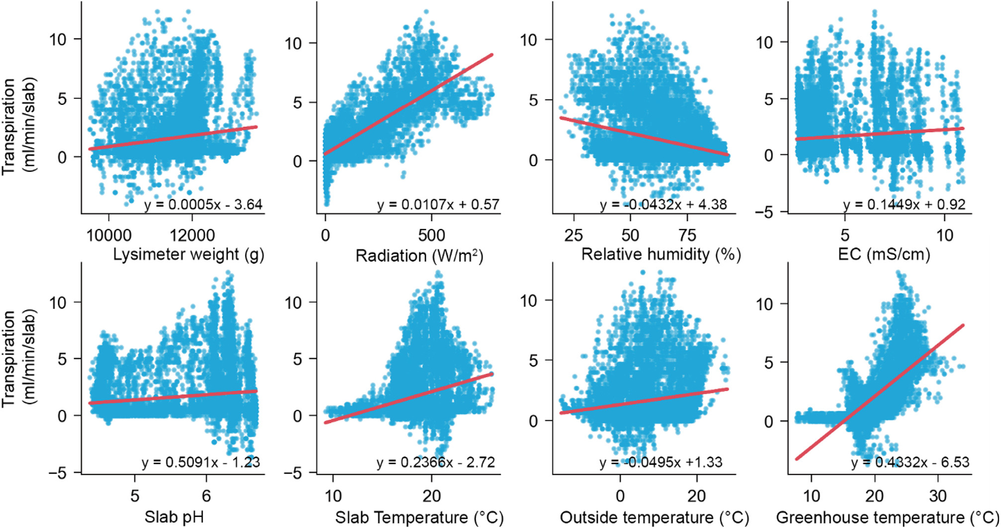
The Pearson correlation coefficient of the variables showed a significant correlation of all measured independent variables (humidity, inside air temperature, outside radiation, EC, pH, slab temp, outside temperature, irrigation, drain, month, and hour) with the transpiration except for day and minute (Table 1). Outside radiation and inside air temperature showed the highest significant positive correlation with transpiration, with correlation coefficients of 0.793 and 0.725, respectively. This indicates that increased outside radiation and inside air temperature can significantly increase transpiration (De Wit, 1958; Jolliet and Bailey, 1992; Zhu et al., 2022). In terms of humidity, a negative correlation shows that an increase in humidity leads to a decrease in transpiration rate (Zhu et al., 2022). The result of correlation analysis was used as a basis for selecting input features for building estimation models to ensure their relevance in predicting the target variables. However, not all variables with significant correlation were chosen for model building. This study considered the first three variables with the highest correlation (outside radiation, greenhouse air temperature, and humidity).
Table 1.
Correlation coefficient of independent variables.
| Variables | Correlation Coefficient |
| Humidity | –0.297* |
| Inside air temperature | 0.725* |
| Outside radiation | 0.842* |
| EC | 0.113* |
| pH | 0.168* |
| Slab temperature | 0.277* |
| Outside air temperature | 0.165* |
| Irrigation | 0.023* |
| Drain | 0.023* |
| Month | –0.188* |
| Day | –0.004 |
| Hour | –0.074* |
| Minute | 0.003 |
Furthermore, air temperature, relative humidity, and radiation are environmental variables that greatly influence crop transpiration (Jo and Shin, 2021). Fig. 1 shows the scatter plot depicting the relationship trend between independent variables and transpiration. In terms of month and hour, despite a significant correlation, the direction of the relationship does not perfectly reflect the actual scenario. Hence, the decision to include these variables, including the day and minute in model building, was based on the observed seasonality of transpiration over time . This is based on the assumption made in forecasting that there is an underlying pattern which described the event and conditions and that it repeats in the future. Identification of patterns and choice of model, particularly in time series, is critical to facilitate forecasting (Nwogu et al., 2016).
2. Comparison of Model Performance
Models built along with the performance evaluation results are shown in Table 2. All models showed potential in estimating transpiration rate using data on radiation, temperature, humidity, and time with R2 values ranging from 0.770 to 0.948 and RMSE of 0.495 mm/min to 1.038 mm/min in the testing. During training and validation, the R2 and RMSE of the models did not go far from each other, with an R2 range of 0.001-0.004 and 0.001-016 for RMSE; hence, overfitting was successfully managed. Early stopping, specifically in the building ANN, LSTM, and GRU models, helped prevent overfitting and reduced its effects on the model (Ying, 2019). For mathematical models, results showed that Polynomial models degrees 2, 3, and 4 have better estimation performance in the testing compared to the MLR model (R2 = 0.77, RMSE= 1.038mm/min), hence showing that the relationship between the independent variables and transpiration is more curvilinear than linear. Among the regression models, polynomial degree 4 (P4) model showed best performance (R2 = 0.93, RMSE = 0.565 mm/min). The polynomial model is useful when the relationship between variables is curvilinear (Ostertagová, 2012).
Table 2.
Model-wise RMSE and R2 values across training, validation, and testing phases.
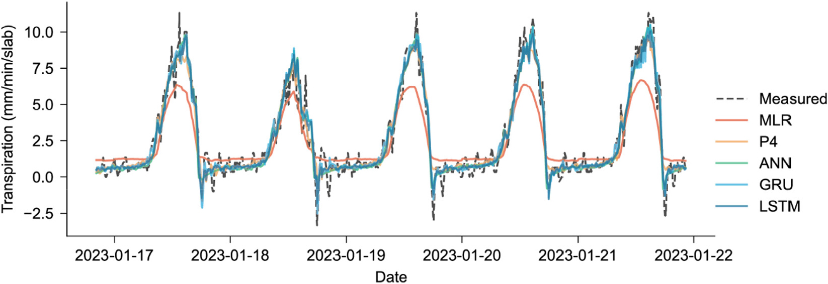
Meanwhile, the performance of deep learning models such as ANN, LSTM, and GRU was better than that of mathematical models. Unlike deep learning models, which do not require knowledge of internal factors and can be constructed with limited data, mathematical models need observation data (Fan et al., 2021). The addition of more relevant input variables can further improve the performance of mathematical models. Fig. 2 shows predictions from January 17 to January 2023, comparing the performance of MLR, 4th degree Polynomial (P4), ANN, GRU and LSTM models. Among all the models, the best performance was observed in the GRU model with R2 of 0.948 in testing and RMSE of 0.495 mm/min. Compared to LSTM, the GRU structure is more concise and has fewer parameters, which minimizes overfitting and improves training efficiency (Li et al., 2022). However, the performance of LSTM and ANN models did not vary much from GRU, which yielded R2 of 0.946 and 0.944, respectively, and RMSE of 0.504 mm/min and 0.511 mm/min. In a study conducted by Chia et al. (2022), it was found that the LSTM and GRU models have tremendous potential in estimating evapotranspiration if just designed with a purpose, such as integrating an optimization algorithm. LSTM and GRU, the ANN model showed promising performance in predicting evapotranspiration in some crops like tomato (Tunali et al., 2023) and paprika (Nam et al., 2019).
The 1:1 comparison of actual transpiration with the transpiration predicted by the models is shown in Fig. 3. The improvement in model performance from MLR to GRU in predicting transpiration can be observed as the distance of the data points got closer to the 1:1 line. However, more dispersed values can be observed in the actual transpiration against transpiration calculated using the PM equation. Similar to the findings of Fernandez et al. (2010), the PM equation underestimated the actual transpiration, as shown by more predicted values that fall far below the 1:1 line. RMSE (0.598 mm/min) offers better performance in prediction compared to MLR and polynomials degrees 2 and 3. However, it has the lowest performance among all models in terms of capturing the variability in the actual transpiration at R2 0.31. Incrocci et al. (2020) explained that PM might underestimate calculation because of the calculation of aerodynamic resistance (ra) as a function of airspeed in the original PM-Eto equation because air movement inside the greenhouses is very low in conditions of natural ventilation, much lower than in open field. To manage this condition, the use of a constant ra value of 295 s/m proposed by Fernandez et al. (2011), which is equivalent to a greenhouse air speed of 0.7 m/s, was adopted in this study. However, contrary to the result of Gallardo et al. (2016), the PM equation still underestimated the actual transpiration. Modification in the equation, such as including other significant factors such as leaf area index (LAI) in the calculation of transpiration (Jo and Shin, 2021), may be done to improve the value of aerodynamic resistance.

In terms of runtime per epoch while building deep learning models, ANN model showed the shortest average runtime per epoch which is 2.16 s, followed by LSTM and then GRU with average runtime per epoch of 47.96 s and 55.29 s, respectively. The architecture of the deep learning models is the same, but sequence lengthwas added to the LSTM and GRU model which contributed to the complexity of these models resulting to longer runtime.
The saved ANN, LSTM and GRU models were used to do forecasting for the next 10, 30, 60, 120 and 180 minutes using unseen data from May 3, 2023, to May 12, 2023. Results of forecasting are shown in Table 3.
Table 3.
Performance of deep learning models in prediction and in 10, 30, 60, 120, and 180-minute forecasting of transpiration.
| Model | RMSE (mm/min) of Forecast | ||||
| 10-min | 30-min | 60-min | 120-min | 180-min | |
| ANN | 4.132 | 517376.018 | -* | -* | -* |
| LSTM | 1.036 | 0.919 | 0.930 | 0.755 | 0.634 |
| GRU | 0.577 | 0.402 | 0.489 | 0.697 | 0.953 |
ANN did not perform well in forecasting compared to GRU and LSTM with RMSE of 4.132 g/min and tremendously increased with increased forecasting time. GRU model showed best performance in making a 10, 30, 60, and 120-minute forecast among all deep learning models with RMSE of 0.577 mm/min. 0.402 mm/min, 0.489 g/min and 0.697 mm/min respectively. LSTM ranked second to GRU with RMSE of 1.036 mm/min, 0.919 mm/min, 0.930 mm/min and 0.755 mm/min respectively. Therefore, for this particular study, GRU is recommended for doing 10 to 120 min forecast but for longer forecasting time (180 min), LSTM is the recommended model. However, performance of deep learning models in doing forecasting should be tested using larger dataset for further verification.
Conclusion
Observed environmental variables which include inside air temperature, outside radiation and humidity were found to have highest significant correlation with transpiration among other variables hence selected as input features for model building. Inside air temperature and outside radiation are found to be positively correlated with transpiration while humidity is negatively correlated with transpiration. Mathematical models such as MLR and Polynomial regression (degrees 2, 3 and 4) modes, and deep learning models such as ANN, LSTM and GRU models were built. All models showed potential in estimating transpiration with R2 values ranging from 0.770 to 0.948 and RMSE of 0.495 mm/min to 1.038 mm/min in testing. Deep learning models were found to perform better in estimating transpiration compared to mathematical models. Among the deep learning models, GRU model and LSTM showed the best performance which both have 0.95 R2 and 0.495 mm/min and 0.504 mm/min RMSE respectively. The FAO56 PM equation underestimated transpiration with RMSE of 0.598 mm/min, which is lower compared to RMSE of MLR and Polynomial degrees 2 and 3. However, it performs the least (R2 = 0.31) among all models in terms of capturing the variability in actual transpiration. In terms of forecasting, GRU model performed better in doing a 10 to 120-minute forecast followed by LSTM while ANN did not perform well in doing longer time forecast. Meanwhile, LSTM performed best in forecasting longer time step. Performance of deep learning models in making forecast should still be done using larger dataset for further verification. Therefore, in this study, LSTM and GRU models are recommended for estimating transpiration of tomato in greenhouse.
