Introduction

Lettuce (Lactuca sativa L.), a vascular plant in the Asteraceae family, originated in Europe and Western Asia and is now cultivated worldwide (NIBR, 2016). With a water content of approximately 95% and a rich supply of vitamins A, B, C, and E, as well as a significant amount of iron, lettuce is considered a crop of very high nutritional value (Jang et al., 2007). Due to these characteristics, consumer demand has steadily increased. In fact, domestic lettuce production in Korea has shown a growing trend, with 95,582 tons in 2019, 96,774 tons in 2020, and 97,137 tons in 2021 (NongNet, 2024). As one of the most consumed raw vegetables, lettuce is an important horticultural crop with continued high demand expected in the future. Kale (Brassica oleracea L. var. acephala), a perennial plant in the Brassicaceae family, has recently gained attention as a “superfood.” It is rich in vitamins A, C, and K, as well as potassium, and contains high levels of antioxidants and dietary fiber, which are associated with antioxidant and anti-inflammatory properties (Satheesh and Fanta, 2020). In Korea, it is primarily consumed in fresh juices and as a wrap. As its consumption as a health food has grown, domestic production has steadily increased, reaching 657 tons in 2021, 845 tons in 2022, and 904 tons in 2023 (KOSIS, 2024). This indicates that kale is progressively establishing an important position in domestic agriculture.

Meanwhile, agriculture must adapt to changing environmental and social conditions to maintain sustainable productivity, which requires rapid and objective decision-making (Hitzler et al., 2021). However, the aging of the rural population is intensifying, leading to a shortage of agricultural labor that directly result in decreased productivity (Heo et al., 2018). In addition, climate change poses a serious threat to agricultural production, causing reductions in yield and quality. According to recent studies, major grain crop yields are projected to decrease by up to 23% under extreme climate scenarios (Rezaei et al., 2023). Climatic factors such as rising temperatures, drought, flooding, and increased salinity also cause direct damage to vegetable production by inducing crop failures, quality degradation, and increased pest and disease outbreaks (Bukharov et al., 2023). Therefore, ensuring the sustainability of agricultural production and responding effectively to these complex challenges require data-driven and objective analysis combined with rapid decision-making, rather than relying on subjective judgment.

Modeling is one alternative to address these challenges. In agriculture, modeling serves as a key tool for increasing productivity and supporting efficient management, and it is utilized in various crop research and cultivation settings. Models based on accurate physiological data can quantify temporal and spatial variability, enabling crop management with relatively less time and lower cost (Gowda et al., 2013). Particularly in the horticultural sector, mathematical modeling using images has been actively investigated, with attempts to predict crop characteristics and yields through regression analysis (Khan et al., 2016; Liu et al., 2013).

Non-destructive regression equation-based approaches offer distinct advantages in agricultural applications. In particular, they enable the acquisition of quantitative measurements without the need for harvesting or damaging the crops, thereby allowing real-time monitoring and facilitating automated crop management. By providing non-destructive and objective measurements, these approaches can directly help mitigate labor shortage issues (Khan et al., 2016). Additionally, the estimation of leaf area and fresh weight can serve as important indicators for evaluating production capacity and optimizing irrigation and fertilization strategies (Karatassiou et al., 2015; Lordan et al., 2015). Recently, research has also shown that 3D modeling techniques integrating 2D images can effectively estimate growth indicators such as biomass, height, and leaf area (Lati et al., 2013).

Therefore, the objective of this study was to develop regression equations to predict the fresh weight (FW) and dry weight (DW) of lettuce and kale using image parameters from top-view (TV) and side-view (SV) perspectives. By comparing the predictive power of TV, SV, and combined TV+SV models, we sought to determine how crop morphology influences the suitability of different imaging angles. Ultimately, the results of this study will provide a foundation for non-destructive biomass estimation strategies for different crops, thereby contributing to the advancement of precision agriculture and automation technologies in the face of increasing labor and climate constraints.

Materials and Methods

1. Plant materials and cultivation methods

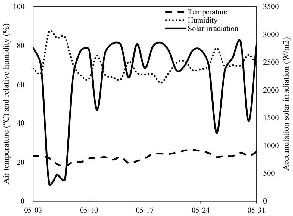
The lettuce cultivar ‘Jincheongmat’ and the kale cultivar ‘Matjjang Kale’ were used. Seedlings, sown on March 16, 2024, were purchased for the experiment. They were transplanted into beds filled with perlite within two single-span plastic greenhouses (designated as Plant Vinyl-34 and Plant Vinyl-35) located at the College of Agriculture and Life Sciences, Chonnam National University (Fig. 1). The plants were transplanted on May 3, 2024, and cultivated until May 31, 2024. The planting densities for lettuce and kale were 9.23 plants/m² and 6.15 plants/m², respectively. A drip irrigation tape with 10 cm emitter spacing was used, and the nutrient solution was periodically adjusted to maintain a pH of 6.0 and an electrical conductivity (EC) of 1.5 mS·cm^-1. Irrigation was supplied every two hours from 09:00 to 15:00, with each application lasting between 1 minute and 30 seconds to 2 minutes. To avoid high-temperature stress, shading was applied daily from 11:00 to 16:00.

Fig. 1

Daily average environment condition.

2. Growth measurement

Growth measurements for both lettuce and kale were conducted at 7-day intervals, starting from the seedling stage. On each sampling date, ten plants were randomly selected from each greenhouse for analysis. The following growth parameters were investigated: number of leaves, leaf length, leaf width, shoot length, stem diameter, leaf area, and the fresh and dry weights of both the shoot and root systems. Shoot length was measured from the surface of the growing medium to the apical meristem of the plant. Leaf length and width were measured on the largest leaf using a ruler; leaf length was measured from the petiole to the tip of the leaf, while leaf width was measured as the longest distance perpendicular to the longitudinal axis. Stem diameter was measured using a digital caliper (CD-15APX, Mitutoyo Corporation, Kawasaki, Japan), and leaf area was determined with a leaf area meter (LI-3100C, LI-COR, Nebras ka, USA). The fresh weights of the shoots and roots were measured using an electronic scale.

3. Image data acquisition and processing

Digital images were captured using an iPhone 14 (Apple, California, USA). Top view (TV) images of the crops were taken in the greenhouse, while side view (SV) images were taken in the laboratory. For scale calibration of the images taken in the greenhouse, a 14 mm × 27 mm pen cap was used. For the images taken in the laboratory, a ruler was used for scale calibration. The background of the plant images was removed using the background removal feature in PowerPoint (Microsoft, Washington, USA). Subsequently, the ImageJ program (1.54k version, National Institutes of Health and University of Wisconsin, USA) was used to calculate the projected leaf area, width, and height from the top view images. From the side view images, the same parameters (projected leaf area, width, and height) were also calculated.

4. Leaf area estimation

The actual leaf area was determined by collecting all leaves from the plant and summing their individual areas. The image-based leaf area was calculated using the ImageJ program. To analyze the correlation between these two measurements, the SAS statistical program (Enterprise Guide v. 8.3, SAS Institute Inc., Cary, NC, USA) was utilized. The results of the analysis were visualized with a scatter plot, and the coefficient of determination (R²) was calculated to evaluate the strength of the relationship.

5. Regression models

After image acquisition, the shoots of the lettuce and kale plants were harvested, and their fresh weight (FW) was measured using an electronic scale. Subsequently, the samples were frozen in an ultra-low temperature freezer (Fre700-90, DAIHAN SCIENTIFIC GROUP, Gangwon-do, Korea) and then completely dried in a freeze-dryer (MCFD8508, ILSHIN BIO BASE Co., Ltd, Gyeonggi-do, Korea) to determine their dry weight (DW). From the images, parameters such as projected leaf area, width, height, and plant height were calculated using the ImageJ program. These image-based data were used as the independent variables, while the measured fresh and dry weights served as the dependent variables. Regression models were developed using Python (visual studio code 1.103.2, python 3.13.2) (Table 1, 2). The models were built separately for each crop (lettuce and kale) and imaging perspective (TV, SV). The predictive performance of each developed model was quantitatively evaluated using the SAS statistical program by calculating the coefficient of determination (R²) and the root mean square error (RMSE).

Results

1. Physiological characteristics of lettuce and kale

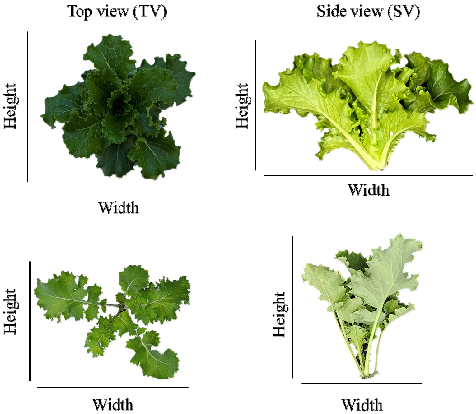
Physiological traits of lettuce and kale were investigated at 7, 14, 21, and 28 days after transplanting (DAT). At each sampling date, twenty plants per species were randomly selected and evaluated for growth characteristics including leaf number, leaf length, leaf width, shoot length, shoot diameter, leaf area (sum of individual leaves), fresh weight (FW), and dry weight (DW) (Table 3). Representative images of lettuce and kale are shown in Fig. 2. Lettuce exhibited a compact rosette structure with wide, horizontally expanded leaves, while kale displayed more upright growth with deeply lobed leaves. These morphological differences are expected to affect the precision of image-based estimations of leaf area and biomass, particularly when comparing top-view and side-view models.

Fig. 2

Morphological comparison of lettuce (top) and kale (bottom) used in this study.

2. Estimation of leaf area

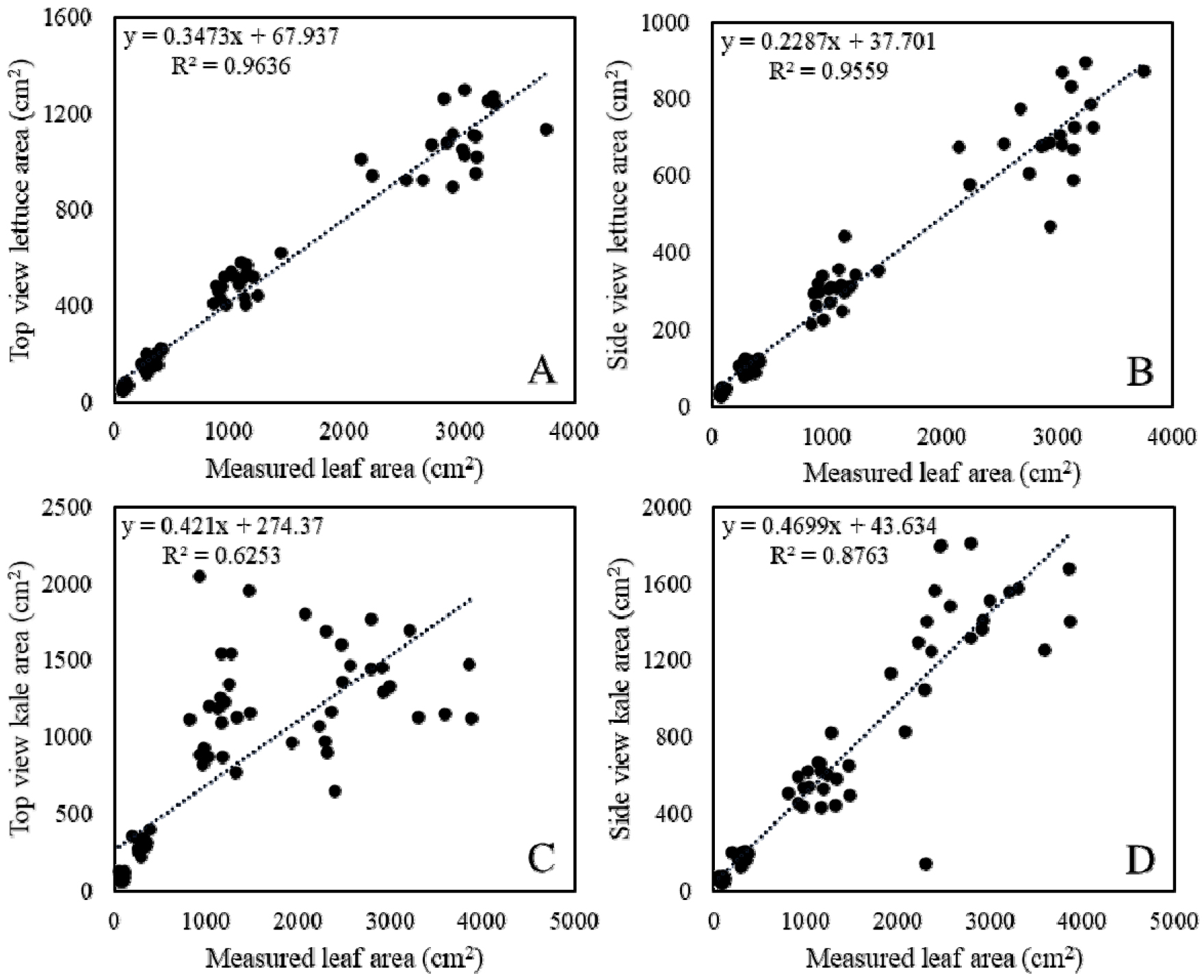
The correlation between the measured leaf area and the image-based projected leaf area was evaluated using scatter plots (Fig. 3). In lettuce, both TV and SV images showed strong correlations with measured leaf area (TV: R² = 0.964, SV: R² = 0.95), indicating that image-derived metrics can effectively estimate canopy-scale leaf area. In contrast, kale showed a weaker relationship in the top view (R² = 0.625), while the side view provided a more reliable estimation (R² = 0.876). These results suggest that crop morphology strongly influences the suitability of different viewing angles for non-destructive leaf area estimation. Specifically, lettuce with its rosette structure can be captured accurately from the top, whereas kale’s more vertical and irregular leaf arrangement requires side-view imaging for reliable prediction. Importantly, the estimation error tended to increase as actual leaf area became increased, suggesting that projection-based approaches are less accurate at later growth stages. This pattern is likely due to overlapping leaves and canopy complexity, which obscure the true extent of the leaf surface area in larger plants.

Fig. 3

Correlation between measured leaf area and image-based estimates using ImageJ. (A) Lettuce (top view, TV), (B) Lettuce (side view, SV), (C) Kale (top view, TV), (D) Kale (side view, SV).

3. Comparison and estimation of FW and DW using top- and side-view models in lettuce and kale

The performance of regression models for estimating fresh weight (FW) and dry weight (DW) varied depending on the crop species and image view (top view vs. side view). To illustrate the range of predictive accuracy, the two best and two worst models were summarized in Tables 4 and 5.

In kale side view models, the R² for DW prediction ranged from 0.859 to 0.941, with corresponding RMSE values between 1.921 and 2.961 g. Similarly, FW prediction models showed R² values from 0.860 to 0.946 and RMSE between 23.614 and 37.982 g (Table 4). These results indicate that, while some regression equations performed poorly, reliable estimation was achievable when appropriate feature combinations were used. In contrast, kale top view models were less reliable, exhibiting poor and unstable predictive accuracy (DW: R² = <0－0.526, FW: R² = <0－0.552) (Table 5). This discrepancy reflects the vertical and irregular leaf architecture of kale, which limits the effectiveness of top-view imaging.

For lettuce side view models, DW prediction showed a wide range (R² = <0－0.933, RMSE = 1.222－4.727 g), while FW estimation also varied broadly (R² = <0－0.913, RMSE = 24.603－83.715 g) (Table 4). Although the lower bound indicates that poorly defined equations may fail to capture the trait, the upper values (DW: 0.933, FW: 0.913) demonstrate that reliable models can still be obtained with careful parameter selection. In lettuce, TV models provided generally robust and reliable predictions. For DW, most TV-based equations showed strong performance with R² consistently above 0.92, highlighting the suitability of the rosette canopy structure for top-view imaging. Although FW models from the TV also yielded slightly lower accuracy compared to DW, the best equations still achieved R² values close to 0.95, indicating that FW can also be estimated with high reliability (Table 5). Overall, these results suggest that TV models are particularly effective for lettuce, with DW prediction being especially stable and FW estimation remaining sufficiently accurate for practical applications.

4. Side- and top-view combined models

When SV and TV parameters were combined, the prediction performance improved compared to TV-only models, particularly in kale. For kale, TV-only models showed weak accuracy (DW: R² = <0－0.526, FW: R² = <0－0.552), but combining SV and TV parameters increased predictive power (DW: R² = 0.828－0.949, FW: R² = 0.851－0.951), with RMSE values reduced by nearly half. However, the performance difference compared to SV-only models (DW: R² = 0.859－0.941, FW: R² = 0.86－0.946) was relatively small, indicating that side-view imaging already captures most of the canopy architecture of kale (Table 6).

In lettuce, both SV and TV models individually showed strong predictive performance (R² > 0.90 for both FW and DW). The combined SV+TV models provided similar or only marginally better accuracy (DW: R² = 0.92－0.973, FW: R² = 0.917－0.935), with minimal reductions in RMSE. This indicates that for lettuce with a rosette-type canopy, TV or SV data alone are sufficient for reliable prediction, and adding both views together does not offer substantial improvement.

5. Selection and validation of optimal regression models

Final regression equations were selected considering three criteria: (i) the highest R² values, (ii) the lowest RMSE, and (iii) acceptable collinearity among predictors (VIF < 10). Based on these thresholds, the best-performing models for kale were derived from combined side- and top-view (SV+TV) parameters, while for lettuce, top-view (TV) models consistently outperformed others.

For kale, the SV+TV models achieved the highest prediction accuracy (FW: R² = 0.951, RMSE = 22.471 g; DW: R² = 0.949, RMSE = 1.786 g), clearly outperforming TV-only models that showed limited reliability (R² < 0.55). This result demonstrates that the integration of both viewing angles compensates for the irregular and upright leaf architecture of kale (Table 7).

In lettuce, TV-based models were sufficient to achieve robust predictions, reflecting the compact rosette structure that is well captured from the top (Table 5). Compared to SV or SV+TV combinations, no substantial improvement was observed, highlighting that additional imaging angles are not necessary for this crop.

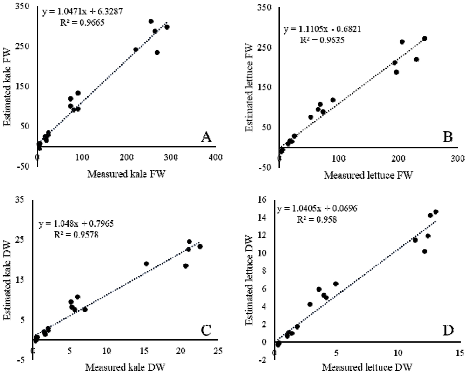
Importantly, the residual patterns revealed some underestimation in the earliest growth stage (7 DAT), particularly in lettuce (Fig. 4B, D), where small plants were sometimes predicted with negative values. This limitation likely reflects the reduced feature variability at early stages, when leaves are too small for stable image-derived predictions. Nevertheless, at later stages (≥14 DAT), both crops showed stable and accurate predictions, which is more relevant for practical applications such as harvest decision-making and yield forecasting, as consumption typically occurs during mid- to late growth stages.

Fig. 4

Scatter plots comparing measured and predicted fresh weight (FW) and dry weight (DW) of kale and lettuce using the selected regression models.

Taken together, these results suggest that SV+TV integration is critical for accurate biomass estimation in kale, whereas TV models alone are sufficient for lettuce. By selecting models with both statistical robustness and biological interpretability, the proposed approach provides reliable tools for non-destructive biomass prediction across crops with contrasting canopy structures.

Discussion

Leaf area is a key morphological trait that influences light interception, photosynthetic efficiency, transpiration, and nutrient response (Blanco and Folegatti, 2005). However, destructive measurement of leaf area is labor-intensive and time-consuming, motivating the development of non- destructive alternatives across many crops (Antunes et al., 2008; Lu et al., 2004; Serdar and Demirsoy, 2006). Likewise, FW and DW are fundamental growth indices: FW reflects water status and marketable yield, whereas DW represents assimilate accumulation and biomass productivity (Poorter et al., 2012; Hatfield and Dold, 2019). Conventional destructive approaches to quantify FW and DW require repeated harvesting and oven-drying, which are impractical for continuous monitoring. Consequently, increasing attention has been directed toward non-destructive imaging and modeling techniques to estimate biomass in horticultural crops (Lu et al., 2019; Yue et al., 2017). In this context, imaging-based regression models provide an efficient alternative for evaluating plant growth.

Several previous studies have demonstrated the feasibility of image-based regression models for estimating plant biomass and structural traits. Hu et al. (2018) estimated the fresh weight of lettuce using three-dimensional point cloud data from a Kinetic sensor and achieved a high correlation (R² = 0.93). Guan et al. (2020) modeled strawberry leaf area and dry biomass from high-resolution RGB and NIR images using object-based image analysis (OBIA) and regression modeling, achieving R² values of 0.79 for leaf area and 0.84 for dry biomass. More recently, Cardenas et al. (2025) applied RGB imaging and machine learning algorithms to predict biomass and leaf area in leafy vegetables, confirming that imaging-derived features can serve as reliable predictors of growth parameters.

Thus, the present study demonstrates that imaging-derived equations can successfully estimate leaf area, FW, and DW while accounting for crop-specific canopy architectures. These findings highlight not only the feasibility of image-based phenotyping for leafy vegetables but also its potential as a reliable research and cultivation tool that reduces destructive sampling and labor demands.

Data availability: The datasets generated and/or analyzed during the current study are available from the corresponding author upon reasonable request.

Ethical Approval: not applicable

Funding: not applicable

Author contributions: Conceptualization, methodology, and supervision, J.S.J.; formal analysis, investigation, and writing—original draft preparation, M.H.B. and I.S.K.; All authors have read and agreed to the published version of the manuscript.

Conflict of interest: The authors declare no conflict of interest.