

Introduction
A crop model is a simple representation of a crop, in general, it is used to study crop growth and calculate the growth of a specific species. There are many crop growth models that simulate physiological development, growth, and yield of crops on the basis of interactions between environmental variables and plant physiological processes (Miglietta and Bindi, 1993;Mo et al., 2005). Recently, crop growth models have been used to investigate the optimal control set points associated with plant factory operations (Ioslovich and Gutman, 2000), and these models have become an essential tool to support field research and to improve agricultural productivity. Also, crop growth models can be used in research, and applications such as yield predictions, agricultural planning, farm management, climatology and agrometeorology (Miglietta and Bindi, 1993).
A closed-type plant factory system is an automated facility for the production of plants; it provides the benefits of consistent production of good quality vegetables, particularly through monitoring the growing conditions of the plants. Proper environmental control is essential for an increase in productivity and quality in plant factories (Morimoto et al., 1995).
Quinoa (Chenopodium quinoa Willd.) seed provides high nutritional values. The leaves and sprouts can also provide high nutritive values, as well as having high antioxidant and anticancer properties (Gawlik-Dzik et al., 2013;Paśko et al., 2009;Schlick and Bubenheim, 1996); hence, there are a number of benefits to using these as vegetables. This experiment was carried out to collect basic data which could be used for the predicting potential effects on the growth rates of quinoa in a closed-type plant factory system.
Materials and Methods
1. Plant material
The experiment was conducted in a closed-type plant factory (700×500×300cm, L×W×H) at Jeju National University. The seeds were sown into 288 cells of a polyurethane sponge (2.5×2.5×2.5cm) in a plastic tray (30×23×6cm), and sub-irrigated once a day with tap water. Emerged seedlings with fully developed cotyledons were sub-irrigated once a day with a nutrient solution with electrical conductivity (EC) of 0.5dS·m-1 and 1.0dS·m-1 at intervals of one week before transplanting. At the fourth true leaf stage, plants were transplanted into plastic plugs in the holes of a trough. The plants were spaced 10cm apart within each trough and troughs were spaced 15cm apart (67plants/m2). Plants were grown in the nutrient solution with an EC of 2.0dS·m-1.
2. Closed-type plant factory system
Three-band radiation type fluorescent lamps (55W, Philips Co., Ltd., Amsterdam, the Netherlands) were used as the light source in the closed-type plant factory system. Light intensity (photosynthetic photon flux density, PPFD) was measured with a quantum sensor (LI-190, Li-Cor Inc., Lincoln, NE, USA), and was maintained at 143μmol·m-2·s-1. The photoperiod was 16/8h (day/night). Temperature was maintained at 23-25°C, and relative humidity and CO2 concentration were 50-70% and 400-600μmol.mol-1, respectively. The nutrient film technique (NFT) system with three layers and four troughs per layer was used for the hydroponic system. Total volume of the nutrient solution in the tank was 90L and the nutrient solution was composed of 15 NO3-N, 1 NH4-N, 1 P, 7 K, 4 Ca, 2 Mg, 2 SO4-S mM·L-1. The EC of nutrient solutions was adjusted by mixing with tap water. The pH and EC of the nutrient solution in each treatment tank were measured daily, using a pH meter (HI 98106, Hanna Instruments Ltd., Leighton Buzzard, Bedfordshire, UK) and a portable conductivity meter (COM- 100, HM Digital Inc., Culver City, CA, USA), respectively. The pH was adjusted to the range of 5.5-6.5 with potassium hydroxide (KOH) or phosphoric acid (H3PO4), and electrical conductivity was adjusted with concentrated nutrient solution or tap water as necessary. The nutrient solutions were supplied via semi-continuous nutrient cycling through the trough with the pump switching on or off every 10 minutes throughout the growing period. Nutrient solution was not renewed during the experimental period.
3. Measurements
Plant growth parameters including plant height, and fresh and dry weight of shoots were measured on 12 plants every 5 days after transplanting. Photosynthetic rate was measured 22 days after transplanting using a portable photosynthetic measurement system (Li-6400, Li-Cor Inc., Lincoln, NE, USA). Plants were randomly selected with 10 replications, and measurements were made on fully expanded leaves.
4. Model construction and validation
Plant height was defined using the following linear and quadratic equations:
| $$\mathrm H=\mathrm a\cdot\mathrm{DAT}+\mathrm b\;\mathrm{or}\;\mathrm H=\mathrm a+\mathrm b\cdot\mathrm{DAT}+\mathrm c\cdot\mathrm{DAT}^2$$ | (1) |
where H is the plant height (cm), DAT is the number of days after transplanting (days), and a, b and c are constants.
Net photosynthetic rate (Pn) was defined with a non-rectangular hyperbola equation and was calculated according to (Goudriaan and Van Laar 1994):
| $${\mathrm P}_{\mathrm n}={\mathrm P}_\max\cdot\{{1-\exp(-\mathrm{αxPAR}/{\mathrm P}_\max)\}}-\mathrm R$$ | (2) |
where Pn is the net photosynthesis rate (μmol·CO2·m-2·s-1), Pmax is the potential photosynthesis rate (μmol·CO2·m-2·s-1), α is the initial gradient under low light conditions (μmol·- CO2·m-2·s-1), PAR is the photosynthetic active radiation (μmol·m-2·s-1), and R is the photosynthesis rate (μmol·- CO2·m-2·s-1) at PAR 0.
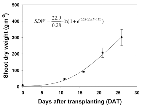
The mathematical function used for expressing shoot dry weight by time is called an expolinear equation (Goudriaan and Monteith, 1990):
| $${\mathrm W}_{\mathrm t}={\mathrm C}_{\mathrm m}/{\mathrm R}_{\mathrm m}\cdot1\mathrm n\lbrack1+\exp\{{{\mathrm R}_{\mathrm m}\cdot(\mathrm t-{\mathrm t}_{\mathrm b})\}}\rbrack$$ | (3) |
where Wt is biomass (shoot dry weight, g·m-2) at t days from transplanting, Cm is the maximum crop growth rate (g·m-2·d-1), Rm is the maximum relative growth rate (g·g-1·d-1) in the exponential growth phase, t is the time after transplanting (day), and tb is the time at which the crop effectively reaches a linear phase of growth (lost time, d).
5. Statistical analysis
The experiment had a completely randomized design. Statistical analyses were carried out using the SAS system (Release 9.01, SAS institute Inc., Cary, NC, USA) and SigmaPlot (Version 9.01, Sistat Software Inc. San Jose, CA, USA). The number of plants for making the plant height model was 16 plants, and the number of validated plants was 144 plants. Variables were estimated using the Gauss- Newton algorithm, a nonlinear least squares technique. The slopes, intercepts and regression coefficients of the models were compared using the SAS REG procedure. Correlation coefficients were calculated between the measured and estimated data.
Results and Discussion
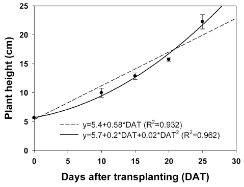
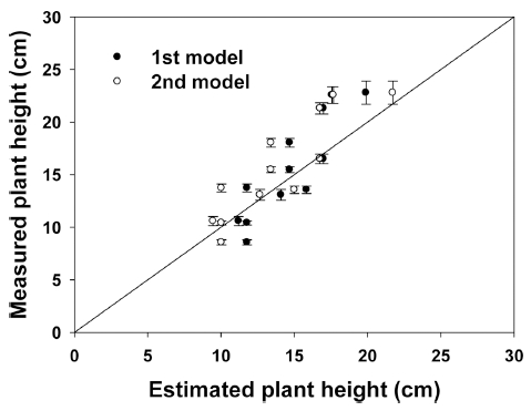
Both linear and curve relationships were observed between the plant heights and days after transplantation (Fig. 1). The plant height model of quinoa was 5.4+0.58·DAT (R2=0.932, P<0.001) or 5.7+0.2·DAT+0.02·DAT2 (R2=0.962, P<0.001), producing a change in plant height of 0.58cm per day or 0.22cm per day. Measured and estimated plant heights were compared (Fig. 2). The linear or curve regression coefficients were 1.07 and 1.12, respectively. The measured and estimated plant heights were shown to be a reasonably good fit with two functions, however, a linear relationship was observed between plant height and days after transplantation. For example, when the distance between the light source and the plants is 30cm, they should be harvested in about 50 days after transplanting. Plant height is one of the most simple and important biomass yield components previous research has shown that increasing plant height is the most obvious and direct way to improve biomass yield for biofuel crops (Salas Fernandez et al., 2009). The potential growth, and hence the potential increase in total biomass, is adjusted daily according to the growth constraints. The adjusted daily total biomass production accumulates through the growing season (Arnold et al., 1995). Therefore, total biomass in closedtype plant factory system could be estimated as plant height.
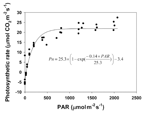
The response of the net photosynthesis rate (Pn) of quinoa to various light levels was measured and modeled (Fig. 3). The non-rectangular hyperbola model (Goudriaan and Van Larr, 1994) was chosen as the response function of net photosynthesis. From our results, the light compensation point was 29μmol·m-2·s-1 and the light saturation point was 813μmol·m-2·s-1 for the quinoa grown for 22 days under a closed-type plant factory system with fluorescent lamps (143μmol·m-2·s-1), and the respiration rate was 3.4μmol·m-2·s-1. The potential photosynthesis rate (Pmax) was 25.3μmol ·CO2·m-2·s-1, and the initial gradient under low light conditions (α) was 0.14μmol·CO2·m-2·s-1. The equation of the non-rectangular hyperbola has frequently been used to describe observed leaf photosynthetic responses to environmental variables (Calama et al., 2013; Cannell and Thornley, 1998; Kim et al., 2004;Lieth and Pasian, 1990;Thornley, 2002).
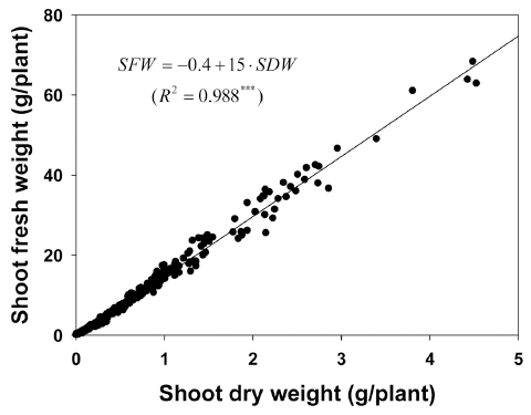
Shoot fresh weight (SFW, g/plant) was shown to be closely related to shoot dry weight (SDW, g/plant), the SFW had a linear relationship with the SDW (Fig. 4). From the model, the SFW was calculated as 15 times the SDW. The measured and estimated SFWs were shown to have a reasonably good fit with this function. Most research on crop productivity has usually concentrated on dry matter, however, fresh weight is of economic interest in the commercial vegetable production sector (Cho and Son, 2009).
A non-linear regression was carried out to describe the increase in shoot dry weight of quinoa as a function of time using an expolinear equation. The maximum crop growth rate was 22.9g·m-2·d-1, the maximum relative growth rate was 0.28g·g-1·d-1 in the exponential growth phase, and the time at which the crop effectively reached a linear phase of growth was 13 days (Fig. 5). The curve of the function indicated a pattern of expolinear growth as suggested by Goudriaan and Monteith (1990). Basically, the growth of crop was exponential with a maximum relative growth rate, and later becomes linear with a maximum crop growth rate. The expolinear growth model as a type of crop growth model has been applied to many crops and has the potential to predict crop growth and yield.
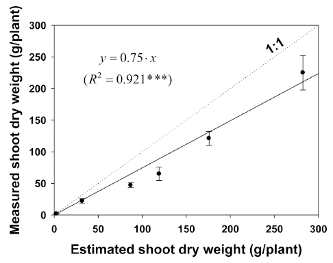
The measured and estimated shoot dry weights were compared (Fig. 6). The regression coefficient was 0.75 (R2=0.921, P<0.001), indicating estimated shoot dry weights were 25% less than the measured values. The measured and estimated shoot dry weights were shown to be a reasonably good fit with this function. The crop yield was calculated as the total dry matter multiplied by the harvest index (Mo, et al., 2005). For instance, with fresh weight per plant at harvest (30g), we can estimate plant height (about 10cm), harvest time (about 18 days), and fresh weight per area (about 2kg·m-2).
It is concluded from this modeling study that growth and yield of quinoa in a closed-type plant factory system respond to photosynthetic active radiation. The non-rectangular hyperbola model was chosen as the response function for net photosynthesis. The modeling growth and yield responses to environmental variables are very useful for the prediction of attainable quinoa yield and to identify the constraints on crop production and management strategies. The results of the present study evidence the importance of continuous research on the economic feasibility for producing quinoa as a leafy vegetable grown in a closed-type plant factory system.
